Using exploratory data analysis, imputation, and machine learning classification techniques, we are tasked with predicting the severity of car accidents (mild or severe) in the United States using a country-wide car accident dataset.
⭐ Link to Kaggle Competition Page ⭐
Abstract
The goal of this project was to predict the severity of car accidents using a provided countrywide traffic accident dataset. Ultimately, our results were submitted to a Kaggle competition where our scores were ranked against our classmates in a 2-lecture wide competition. This dataset was extremely large, with a comprehensive 50,000 observations recorded over both a training and testing dataset. We were tasked with creating multiple predictive models based on provided and independently-developed predictors to attempt to achieve a high score on Kaggle – essentially how well our predictions match the real ‘test’ classifications. Our final model was a Random Forest model that produced a final score of 0.9355 – to earn us a score of 14th in our lecture.
Introduction
There are on average 6,000,000 car accidents in the US every year. In just an instance, ordinary people can be left devastated – from thousands of dollars lost in repair costs to more horrific outcomes like paralysis, death, or loss of a loved one. Many causes can lead to car accidents, including people driving under the influence, driving while texting, or weather conditions. While recognizing the causes of accidents, it is also interesting to think on the flip side – what are the effects of car accidents on surrounding areas? Here we look to answer that question, specifically, what is the effect of a car accident on traffic – measured as “MILD” or “SEVERE”. Thus building a predictive model to successfully predict the severity of car accidents based on traffic conditions is critically important for public safety. In this Kaggle project, we examine a US countrywide traffic accidents dataset from 2016 to 2021. The data on traffic accidents are being collected through APIs which provide streaming traffic incident data. The original training dataset has 35,000 observations, and the testing dataset has 15,000 observations. There are 43 predictors we look at to predict the ‘Severity’ response variable, including properties of car rides which are both numerical and categorical. The numerical variables predictors include temperature outside, distance of car ride, and feature engineered predictors like the time length of car ride. The categorical variables predictors include predictors like the city of car accident, whether there was a junction at the car accident, and feature engineered predictors like whether the term “caution” was in the description column of the dataset. We aim to build a classification model that can predict the response variable ‘Severity’ in the testing data by selecting key predictors to build the most accurate model.
Exploratory Data Analysis and Data Cleaning
A. Understanding the Structure of the Data
Without any modifications, the original dataset contained 11 numerical variables and 32 categorical variables. We first took a look at the categorical variables:

Here we saw that some of the categorical variables contained far too many levels for us to work with, with many variables nearing 35,000 levels (roughly one level per observation). So, before building the model, we would have to reduce the number of levels for those predictors.
After that, we took a look at the numerical predictors. While many of them were self-explanatory and didn’t need any adjusting, we saw that some of them had potential to be highly correlated, which would increase the complexity of our model without providing much additional information. Those variables were those that had a start and end, such as Start_Lat and End_Lat. In order to best optimize our model, we would have to reduce the collinearity between those variables, as well as reducing multicollinearity between the categorical variables as well.
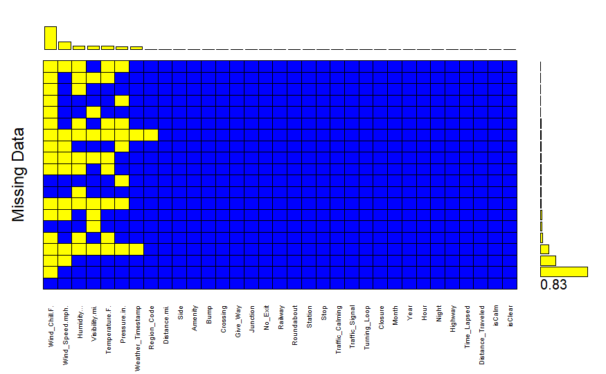
The last thing we did before cleaning the data was looking at the structure of missing values in the dataset as follows:

There were 13,211 missing values in the original dataset, but only 17 variables accounted for all of them. Based on the plot, we observed that the majority of those variables were weather-related, which raised questions about the data collection process since weather variables weren’t strictly being recorded. That being said, all of those predictors had less than 20% missing values, so we proceeded with imputation to fill in missing values.
B. Dealing with Categorical Variables
The first categorical variable we dealt with was the Description variable. With 31,058 levels and no strict sentence structure, we created word clouds of the severe and mild car accident descriptions separately to observe any differences between them.
| Severe Accidents | Mild Accidents |
|---|---|
 |
 |
While words like “accident” and “exit” appear in both word clouds, words like “closed,” “road,” and “blocked” appear more often in severe accidents than mild ones. So, we created 11 dummy variables for the words that stood out most to replace the description variable.
The next variables we looked at were the Start_Time, End_Time, and Weather_Timestamp variables. All three of these variables were time related, and followed a specific structure for each observation. First, we extracted the hour, month, and year values out of the End_Time variable using regular expressions, as these variables started off as character strings. After that, we converted the three variables into POSIX format, which is the number of seconds since January 1st, 1970. Finally, we created a Night variable, which is a binary variable indicating whether or not the accident took place between the hours of 7pm to 7am.
For the Wind_Direction variable, we noticed that there were a lot of repetitive levels (e.g. “East” and “E”). So, we combined those repeated levels, which reduced the number of levels from 24 to 18. This was still a high amount of levels, however, and so rather than looking at the direction of the wind, we created a dummy variable called isCalm which indicated whether the Wind_Direction was “Calm” or not. We did the same thing with Weather_Condition by creating a isClear variable, indicating whether the Weather_Condition was “Clear” or not.
For the Zipcode variable, we decided to narrow down the original 15,863 levels down to 10, as we created a new variable, Region_Code, that took the first digit from each Zipcode. We did this because the first digit of every Zipcode represents a region in the United States, such as the West Coast for 9 and New England for 0.
The last categorical variable we looked at was the Street variable. We reasoned that if the accident took place on a highway, it would more likely be severe since driving speeds are much higher on average. So, we created a new variable called Highway that indicated whether the Street variable contained “Hwy,” “Highway,” or “I-.”
After creating all of these variables, we removed the original variables that contained too many levels, allowing us to preserve as much information as possible without retaining the highly-complex categorical variables.
C. Dealing with Multicollinearity
As mentioned earlier, there were some variables that we felt could be highly correlated, especially variables with a “start” and “end.” The first one we looked at was the Start_Time and End_Time predictors, which we thought were correlated with the Weather_Timestamp variable as well. Since we converted them into POSIX format in the previous part, we could now take the difference between the two to create a Time_Lapsed variable, which measures the duration of each accident in seconds. Similarly to the Start_Time and End_Time predictors, we created a Distance_Traveled predictor by calculating the euclidean distance between the Start_Lat, End_Lat, Start_Lng, and End_Lng variables. After that, we noticed that the variables Sunrise_Sunset, Civil_Twilight, Nautical_Twilight, and Astronomical_Twilight all measured the same thing as our new Night variable using different metrics. So, we combined these 5 variables into a single Night variable by taking the majority value for each observation. Finally, we removed the correlated variables discussed in this section, leaving us to deal with missing values.
D. Dealing with Missing Values
After completing the steps in parts B and C, we looked at the missing values once again:

Just by cleaning the data, we were able to reduce the number of variables with missing values to six. With that in mind, we proceeded to imputation.
To impute the missing values, we used the Hmisc library’s aregImpute() function, which uses additive regression, bootstrapping, and predictive mean matching to impute missing values. The benefit of this approach is that it works for both categorical and numerical variables and results in zero missing values. One of the downfalls of this approach, however, is that this approach assumes the variables with missing values are linear, which may not be the case for all of those predictors. Since most of the predictors had less than 5% missing values, we decided that the benefits outweigh the cons and proceeded with predicting the severity of car accidents.
Building the Model
To build our car accident severity model, we trained on our models using the predictors and labels provided by the testing data in Kaggle. From there, we use the predictors from the testing data from Kaggle to make our predictions on the observations. We applied these steps to build our three different classifiers: KNN, XGBoost, and Random Forests. We then compare these models and select the highest accuracy and best performing model.
A. K Nearest Neighbors (KNN)
KNN is a simple and very interpretable classification algorithm that computes Euclidean distances among predictor variables under the principle that data follows similar data. In practice, this means that a data point is classified based on the majority vote of the nearest K data points. We implemented KNN with different values of K.
| K-Value | Test Accuracy |
|---|---|
| 10 | 87.41 |
| 25 | 88.08 |
| 50 | 89.28 |
We observe that accuracy increases with higher values of K. However, all three models scored with accuracy less than 90% on the testing data, indicating that KNN models are too complex and not a good fit for the dataset we are using.
B. XGBoost Classifier
Extreme Gradient Boosting (XGBoost) is a classifier algorithm that minimizes the loss function of traditional boosting by combining weak learners. It is similar to Gradient Boosting, except it uses advanced regularization techniques (L1 & L2) to prevent model overfitting and drive more accurate results. This model scored an accuracy of 92.02% on the testing data. The feature importance plot is shown below:

This model shows us that XGBoost is great for unbalanced, sparse datasets as it is more efficient due to self-tuning, performing better than our KNN Classifier. However, we believe this is not the optimal model and our accuracy can still be improved.
C. Random Forest Classifier
Random Forest is an ensemble classification technique that combines the results of multiple decision trees trained on subsets of data generated by the bootstrap technique, meaning samples are drawn with replacement from the training data. This technique aims to reduce overfitting by reducing variance and correlation between decision trees. We first aimed to optimize the number of predictors used in our Random Forest model by adjusting for the mtry hyperparameter in our model.

We determined that 37 predictors is the optimal amount of predictors to use in our model (mtry = 37) and this gives us the best accuracy of 93.53% on the testing data.

Furthermore, the feature importance plot above shows us which predictors are critical in building our random forest model with Weather_Timestamp, contains_road, and contains_due being key variables to name a few. This is the highest performing model.
D. Model Building Summary
We have built three different classifiers to predict the severity of car accidents. We can compare and contrast the results our models with the visualization below:

Ultimately, the Random Forest Classifier performs the best, seen with the highest accuracy on the training data. While trying other classification techniques like Logistic Regression and KNN, Random Forest has the following benefits that make for a better model – versatility to data (multiple decision trees are fit), high interpretability (with the variable importance plot), and being a powerhouse in prediction performance.
Limitations
While we are proud of the model we constructed, we also recognize that there are multiple limitations to our model and methodology that are worth noting. If we were able to do this project again, there are a couple areas where we may have approached the solution differently or areas where we would’ve shifted our focus.
In regards to the model construction and data cleaning, there are a couple of points worth noting where our process could have been improved. In general, we took an approach of extracting the most valuable information from various provided predictors to create our own – either in the form of dummy variables, substring data, or finding the difference between two column values. For example, when looking at the text mining approach we took with the ‘Description’ variable, we created 11 dummy variables that identified the presence (or lack thereof) of a specific word in each description. While this allowed us to remove the original ‘Description’ predictor with over 30,000 levels, we also cannot be fully confident that our new variables best capture the original information provided. Would we have been better off adding more dummy variables? Should we have looked for phrases instead of simply words? These are examples of questions we should ask ourselves in review of our model. In general, we believe that we successfully extracted some of the most relevant information from the original dataset – nevertheless, we recognize the room for improvement.
When imputing the data, as expected, we also faced some limitations in regards to maintaining the authenticity of the original data without significant adjustment of our own. Using the Hmisc library’s aregImpute() function to impute missing values, we were able to find an approach that takes care of missing values for both our categorical and numerical predictors. After researching other methods, we recognized that this function took multiple valuable steps in the process of imputing data – under the assumption that the variables with missing values are linear. This is a strong assumption to make that we still cannot guarantee is necessarily true for every predictor. Additionally, with imputing values of variables with a larger amount of missing data (generally weather predictors), we weren’t able to use other predictors as context in this imputation. For example, maybe the ‘Description’ variable would occasionally hold information regarding the weather conditions when that data isn’t recorded – and as a result, our imputed weather data may have been inaccurate. Nevertheless, this process would have been tedious and outside of our general skillset and timeframe. Ultimately, while our process of imputation may not have been perfect, limitations here are inevitable. We believe the Hmisc library did the most effective job of producing a holistic dataset representative of our original data.
While our Random Forest model ultimately achieved the best results, it does come with limitations of its own – namely how computationally expensive and the potential for overfitting. Furthermore, in general the Random Forest approach is less interpretable than other model methodologies. The algorithm works as a black box where we have little control beyond adjusting a couple of parameters. In our specific approach, we could have improved by better utilizing the Variable Importance Plot. Here, we could have recognized some predictors that were less relevant to the data and thus causing overfitting. Some of these predictors may have been redundant given the high number of features in our final model. Pruning would have been a good approach to attempt in retrospect when looking at our model results.
Finally, we also recognize that features not listed in the data may have been effective predictors to classify this dataset. The use of external data is definitely something we believe could have helped improve our model – whether that be population data to recognize denser streets across the country or more detailed data to describe road conditions. In the process of restructuring data, imputing missing values, constructing the Random Forest model, or not taking advantage of external data, there are many limitations worth noting and ways we could have improved our methodology. Nevertheless, our final model was accurate, effective, and successful in predicting the severity of car accidents.
Conclusion
As we created a model to predict and classify the severity of car accidents around the country, our team thoroughly enjoyed this project and learned from every step of the process. In the act of cleaning and restructuring the data, imputing missing values, testing different predictive models, tuning our Random Forest Classifier, recognizing our limitations and drawbacks, collaborating as a group, conveying our methodology in a presentation, and even in writing this report, us three have greatly appreciated our results and the hard work we committed to this project. The bounds of learning for this competition were endless – while also giving us the healthy motivation to continuously improve to perform better than our peers. Our final model was a Random Forest Classifier built on 44 predictors, with an mtry value of 37. Ultimately, our final model accurately captured the true class of 93.55% (0.9354 PUBLIC score and 0.9357 PRIVATE score) of the 15,000 test data observations. While we ranked 14th place in our lecture at 23rd overall, we are proud of our model and accuracy we achieved in predicting the severity of car accidents. We are greatly appreciative of our professor, Prof. Akram Almohalwas, in his support throughout this process and for this opportunity.