VALORANT Ranked Analysis
Personal Note
VALORANT was initially released as a closed-beta experience in 2020, which was exciting as the creators of one of the world’s most successful Esports, League of Legends, developed a game that would directly compete against Counter Strike in the tactical first-person shooter (“tac FPS”) genre. I was immediately hooked, participating in collegiate events, but I knew there was a competitive professional scene with jaw-dropping tournament prize pools and notable salaries just beyond the horizon.
Years before, I devoted hundreds of hours to a similar game by Valve—Counter Strike: Global Offensive. Just like VALORANT, there existed a professional scene teeming with the world’s best players and it was my dream to compete in front of hundreds of thousands of fans in sold-out stadiums. At the time, that dream was more of a fantasy and I shifted my focus on other things, but with the release of VALORANT and the COVID-19 pandemic coinciding, I reignited my passion for Esports and progressed to the top 0.05% of all players by rank while juggling school and my career. As I got closer to my graduation date, I realized two things: first, that based on my capabilities playing recreationally, I had a chance of seizing my childhood dream if I’d fully committed to playing full time and second, I’d only get this opportunity while I was young.
For this reason, after graduating in the Summer of 2024, I set aside a year to work towards achieving the highest rank, Radiant, and practicing with other teammates for five-seven hours a day to try to go pro. I knew it was a longshot, but I also knew I would always ask myself “what if?” for the rest of my life if I didn’t make an honest attempt.
Hence, the art of improving and climbing to the highest levels of VALORANT is near and dear to my heart, and this project represents a celebration of my attempt and the gratification of my child-self’s dream. This project combines everything I love: competition, data, and insight. It’s not just an analysis of numbers. It’s a reflection on performance, learning, and playstyle—mine and others’. I appreciate anybody reading this and I hope you learn a thing or two! :)
1. Abstract
This project explores what differentiates top-ranked VALORANT players using statistical analysis, clustering, and predictive modeling. I scraped and analyzed data from 292 players—roughly the top 50 from six regions—applying KMeans clustering and PCA to uncover three playstyle archetypes: “All Aim, No Brain,” “Support,” and “Balanced.” Supervised models were trained to predict rank rating (RR) and win rate, with Ridge Regression achieving an R² of 0.47 for RR and XGBoost reaching 0.62 for win rate. SHAP-based feature importance revealed that less conventional metrics—such as 1v2 clutches lost, match duration, and legshots dealt—were more predictive of success than commonly emphasized stats like average combat score, headshot percentage, or average damage. Notably, KAST, a widely used metric in pro-play analysis, emerged as a strong predictor of win rate. Findings across models and clusters also suggested that supportive playstyles, while valuable to team dynamics, tend to be less effective for climbing in ranked where measurable individual impact is more heavily rewarded. Personalized SHAP visualizations further enabled player-specific feedback, offering individualized insights for improving ranked performance.
2. Introduction
The ranked system of Riot Games’ competitive first-person shooter game, VALORANT, is predominantly determined by each player’s capacity to win matches. Simply put, after obtaining an initial rank, players rise or fall through various ranks (Iron, Bronze, …, Immortal, Radiant) as they continue to win or lose ranked games. While there are several other factors contributing to how much rank rating (RR) each player receives or loses per match, a player is guaranteed to climb to higher ranks so long as they win.
Winning, however, is easier said than done. Because of the five-versus-five format and a match-making system that puts players of similar skill levels against one another, the likelihood of winning approaches 50% as players plateau into a rank where they can’t seem to push past, also known as being “hardstuck.” Players’ ranks fall under a roughly Normal distribution, as seen in Figure 1, with an average rank around Silver and Gold. More skilled and knowledgeable players can significantly impact their games before settling at higher ranks, but unlike the rest of the ranks, the highest rank, Radiant, has no RR ceiling. So, even among the top 0.01% of players who manage to hit Radiant, there are some players who accumulate up to seven ranks worth of RR over those who barely scrape by. Some are professional players, some are streamers, and some are simply hobbyists, but in the VALORANT community, they are commonly known as “ranked demons.”
Figure 1. Ranked distribution for V25 Act II
The goal of this project is to determine what traits these so-called “ranked demons” possess that set them apart from the rest of the playerbase. In other words, how are they able to consistently tilt the balance of a ranked game in their favor and does that ability look different depending on region, playstyle, or role? To explore this, the project focuses on four main objectives: (1) identify the gameplay statistics that most strongly distinguish top-ranked players from each region, (2) cluster players based on their stat profiles to uncover emergent playstyle archetypes, (3) predict ranked success, measured by both rank rating and win rate, from performance data, and (4) apply these same tools to evaluate my own performance and that of my friends to see where we stand in comparison.
3. Data Sources
This project uses publicly available player statistics from Tracker.gg, a third-party site that aggregates VALORANT match data and performance metrics. While Riot Games offers a developer API, access to match history and player stats is restricted to approved production projects, so web scraping was used as an alternative method for data collection.
The dataset includes the top 50 ranked players from six major regions: North America (NA), Europe (EU), Asia Pacific (AP), Korea (KR), Brazil (BR), and Latin America (LATAM)—totaling an initial target of 300 players. These players were selected directly from each region’s leaderboard using automated scraping scripts, which also captured their extended stat breakdowns by clicking into each profile’s detailed “Show More” section.
In addition to leaderboard players, the dataset includes my own VALORANT stats as well as those of several friends, collected using the same pipeline. This allowed for direct comparison against top-tier players using consistent metrics and preprocessing.
Due to the nature of web scraping, several limitations arose during collection:
- Page load delays, rate limits (HTTP 429 errors), and CAPTCHAs occasionally blocked access
- Some pages failed to fully compile player data before being parsed
- Incomplete stat panels or unexpected page structures led to missing values
After accounting for these issues, I successfully collected 292 complete player profiles out of the original 300. These players form the foundation for all subsequent analysis in this project.
4. Exploratory Data Analysis (EDA)
To better understand how player performance differs across regions, I conducted exploratory distribution analysis on several key gameplay metrics. The goal was to identify whether certain regions demonstrated statistically distinct playstyles or competitive profiles, and whether any features were potential early indicators of regional trends or imbalance.
The following features were selected for regional comparison due to their relevance in measuring combat effectiveness, consistency, and overall impact in ranked games:
Selected Features:
- Rank Rating (RR)
- Average Combat Score (ACS)
- KAST
- Damage Delta (DDΔ)
- Damage per Match
- Entry Success Rate (ESR)
- First Bloods per Match
- Headshot Percentage
- KD Ratio
- KDA Ratio
- Kills per Match
- Time Played
- Round Win Rate
- Game Win Rate
Within most of these features, the distributions appeared broadly consistent across each of the six regions. For example, side-by-side boxplots of ACS per region showed relatively consistent ranges, medians, and interquartile spreads with a slightly elevated distribution for Korea (kr) as seen in Figure 2. Metrics such as KAST, KD ratio, and kills per match showed comparable trends, suggesting that high-level players across the globe generally meet similar statistical thresholds for combat performance. However, few features stood out as notable exceptions, including rank rating, damage delta, and time played.
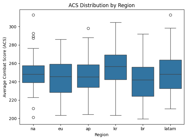
Figure 2. ACS distribution by region
One of the most pronounced differences appeared when looking at the distributions for rank rating in Figure 3. The Korean region displayed a significantly lower RR distribution than other regions despite these players being ranked among the top 50 in their region. Table 1 shows the five-number summaries of these distributions, illustrating how Korea’s RR distribution is lower than all of the other regions in every regard, such as the median RR value of 492 being almost half of the median RR value for the neighboring Asia-Pacific region.
Figure 3. Rank rating distribution by region
Table 1. Five-number summaries for RR by region
| Region | Minimum | 25% | Median | 75% | Maximum |
|---|---|---|---|---|---|
| Asia-Pacific (AP) | 870 | 906 | 969 | 1042 | 1244 |
| Brazil (BR) | 699 | 762 | 837 | 897 | 1174 |
| Europe (EU) | 887 | 907 | 927 | 978 | 1117 |
| Korea (KR) | 407 | 445 | 492 | 562 | 903 |
| Latin America (LATAM) | 586 | 628 | 684 | 745 | 1029 |
| North America (NA) | 770 | 808 | 856 | 930 | 1126 |
A similar regional skew was observed in the damage delta (DDΔ) and time played variables. Note that damage delta is somewhat correlated with time played, as skilled players regularly deal more damage to their opponents than they receive and that damage accumulates as they play more games. Once again, however, Korean players exhibited notably lower time played (and hence damage delta) values compared to their counterparts in other regions (Figure 4 & 5), but not as significant of a difference as their RR values. While players are required to grind more hours to build RR overtime, it appears that many Korean players are still spending enough time to be competitive with other regions, suggesting that the differences in RR distributions may be attributed to other factors. In fact, when looking at game win rate, which is not influenced directly by play time, I saw that Korean players are well within the standard ranges displayed by other regions (Figure 6). Hence I continued to look for potential differentiating factors that set the Korean region apart in terms of RR, but also looked for other factors that affect win rate over all.
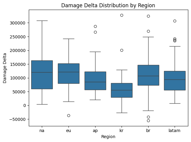
Figure 4. Damage delta distribution by region
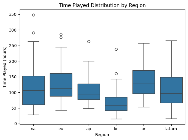
Figure 5. Time played distribution by region
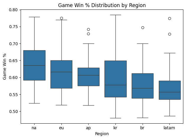
Figure 6. Game win rate distribution by region
5. Data Preparation
Before performing any clustering or modeling, I cleaned and standardized the dataset to ensure consistent and reliable input features. This involved addressing missing data, transforming feature formats, and applying standard preprocessing techniques commonly used in machine learning workflows.
5.1 Handling Missing and Incomplete Data
Some player profiles were only partially available due to incomplete page loads or missing stat panels during the scraping process. These entries were filtered out, resulting in a final dataset of 292 complete player profiles. Additionally, individual features with missing or blank values (e.g., “—” or empty strings) were cleaned and converted to NaN, and rows containing critical missing fields were excluded.
5.2 Correcting Feature Names and Values
Tracker.gg reports statistics with a mix of inconsistent formatting (e.g., “Ability 1 Casts / Match”, “K/D Ratio”, “Damage Delta δ”). To streamline the analysis and make column names code-friendly:
- Lowercased all labels
- Replaced spaces/special chars with
_ - Converted percentages, times, and numbers appropriately
On top of that, several stats were stored as strings due to formatting on the source website:
- Percentage values (e.g., “48.7%”) were converted to decimals (e.g., 0.487)
- Comma-separated numbers (e.g., “1,234”) were parsed into integers
- Time-based features (e.g., “32m 34s”) were converted to total seconds for consistency
This allowed for uniform access across the pipeline, easier visual interpretation of feature names, and appropriate value types for analysis.
5.3 Feature Scaling and Normalization
To prepare the data for clustering and regression models, all numerical features were standardized using StandardScaler from scikit-learn. This transformation ensures each feature has zero mean and unit variance, which is especially important for distance-based algorithms like PCA and KMeans.
5.4 Feature Selection: Redundancy Removal
To reduce noise and avoid redundancy, I filtered out:
- Removed low-variance features
- Removed highly correlated features (r > 0.95)
The original dataset contained 153 features per player. After completing the steps above, I reduced the number of features to 73, resulting in a dataset that maintained a rich, diverse set of informative features while improving interpretability and computational efficiency.
6. Methodology
To better understand player performance in VALORANT, I applied a combination of unsupervised and supervised machine learning techniques. First, I used dimensionality reduction and clustering methods to uncover latent playstyle archetypes among top-ranked players. This helped surface groupings such as fraggers, support players, and more balanced hybrids, based purely on gameplay statistics. Next, I trained predictive models to estimate a player’s rank rating (RR) and win rate from their stat profile. These models not only quantified feature importance, but also enabled personalized evaluations using tools like Shapley Additive Explanations (SHAP), which highlight how specific performance metrics contribute to a specific player’s success or shortcomings.
6.1 Clustering
To conduct clustering, I used KMeans clustering on our processed dataset as our scaled variables were now appropriate for distance-based analysis. I applied clustering nine times using different numbers of centroids per iteration, then used the elbow method to determine the optimal number of centroids. After selecting an optimal fit, I evaluated the most prominent features in each cluster by comparing their z-scores and labeled each cluster with an appropriate descriptor.
For visualization purposes, I then applied two-dimensional PCA to reduce the 73 features into two principal components. In doing so, I was able to plot the players on this new PCA space to visualize the distinction of clusters.
6.2 Predictive Modeling
To quantify which gameplay statistics most strongly influence ranked success, I trained several regression models to predict rank rating (RR) and win rate from players’ stat profiles. These models provided a framework for both evaluating predictive accuracy and interpreting which features contribute the most to performance outcomes, i.e. which stats really matter.
I selected a diverse set of algorithms that reflect different modeling paradigms:
- Lasso Regression: A linear model with L1 regularization, which can shrink some coefficients to exactly zero, effectively performing feature selection
- Ridge Regression: A linear model with L2 regularization, which shrinks coefficients to reduce overfitting but retains all features
- Random Forest Regressor: An ensemble of decision trees that captures non-linear interactions and is robust to outliers and multicollinearity
- XGBoost Regressor: A gradient boosting method that builds trees sequentially and optimizes for residual error, often outperforming Random Forest on structured data
Each model was trained using an 80/20 train-test split with light hyperparameter tuning on the following hyperparameters using cross-validation for single parameters and GridSearchCV on multiple parameters:
- Ridge/Lasso: regularization strength alpha
- Random Forest: number of trees, max depth
- XGBoost: learning rate, number of estimators, max depth
To evaluate these models, I used R2 score, Root Mean Squared Error (RMSE), and Mean Absolute Error (MAE).
6.3 Feature Importance
Beyond model performance, a key goal of this project was to understand which gameplay features contribute most significantly to a player’s success in ranked VALORANT. To do this, I examined feature importance using the multiple modeling approaches above, each offering a different lens on the data.
For linear models like Ridge and Lasso, feature importance was derived from the magnitude of the model coefficients after standardization. In Ridge regression, all features are retained and the coefficients indicate the relative weight of each variable under regularization. Lasso regression, by contrast, imposes stronger sparsity through L1 regularization, often shrinking some coefficients to zero entirely. This makes Lasso particularly useful for isolating a smaller subset of features that are most critical, while Ridge provides a broader view of contributing variables. Tree-based models such as Random Forest and XGBoost offer model-specific feature importance measures based on how frequently a feature is used to split data and how much it reduces error.
To enhance interpretability and move beyond global averages, I also used SHAP (SHapley Additive exPlanations) values, which are model-agnostic and provide instance-level explanations. SHAP values decompose a model’s prediction for a single data point into additive contributions from each input feature, allowing for a more nuanced understanding of how and why a particular prediction was made. This is especially valuable for more granular evaluation as it sheds light on the strengths and weaknesses of each individual, rather than a group of players.
Taken together, these complementary methods offered both global and local insights, providing transparency into the decision-making process of each model and laying the groundwork for personalized evaluation and comparison.
7. Cluster Analysis
After fitting nine different KMeans algorithms, ranging from two centroids to ten, I observed the inertia values per iteration and visualized them in Figure 7. Since there was no clear “elbow,” a point where the change in inertia significantly decreased, I chose three clusters to simplify our analysis for easier interpretability. This also allowed us to maintain at least 50 players per cluster, as a fourth cluster would’ve resulted in 39 players which is arguably too small of a group to observe notable differences. With three clusters, each cluster was made up of 60, 98, and 134 players, resulting in large enough groups with significant boundaries.
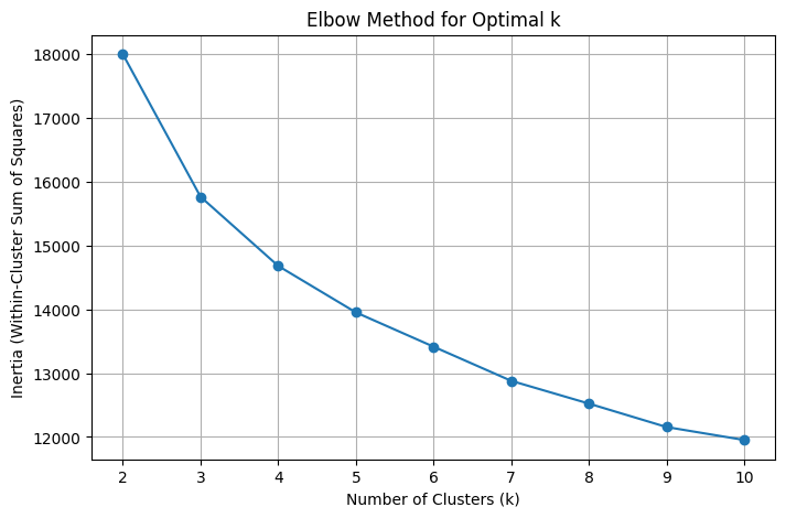
Figure 7. Inertia vs. cluster count
Upon assigning clusters to each player, I computed the z-scores of the average values per feature within each cluster. This allowed us to see which cluster-specific variables deviated from the other clusters the most by evaluating the z-scores with the greatest magnitude, effectively giving us a list of each cluster’s most distinctive features. A snapshot of the results are in Table 2, and using these results, I labeled the clusters appropriately.
Table 2. Top 5 traits per cluster
| Cluster | Highest | Lowest |
|---|---|---|
| Cluster 0 | First bloods, 3Ks, Headshots, 4Ks, Kills | Clutches, Grenade casts, Round duration, Defuses, Ability 1 casts |
| Cluster 1 | Ultimate casts, KAST, KAD, Damage delta, Ability 1 casts | Ability 2 casts, Assists, Deaths, Assists, Plants |
| Cluster 2 | Assists, Plants, Match duration, Ability 2 casts, ACS | RR, First bloods, Ultimate casts, Damage delta, Match duration |
Cluster 0 is characterized by players with high fragging abilities (first bloods, 3Ks, headshots, et cetera.) and lower supporting traits. Fewer clutches may seem like an odd distinction for players who are mechanically talented, but it is likely due to the fact that these players seek gun fights earlier into the rounds and are rarely the last ones alive. Similarly, these players are less likely to use supporting utility like grenades and abilities, are more likely to immediately shut down rounds on their own, and are less likely to be alive for spike defusals. For these reasons, I labeled this cluster “All Aim, No Brain” (AANB) to highlight its players’ mechanical skills and lack of team play potential.
Cluster 1 players are much more balanced than those in Cluster 0. Their biggest defining factor is their ultimate ability usage, signifying an awareness and mastery of the utility side of the game while maintaining strong mechanical skills as indicated by their high KAST, KAD, and damage delta values. They’re likely not the first player to engage in a fight, but are able to support and, more importantly, capitalize on the opportunities generated by their entry fraggers. While playing a slightly more supportive role than Cluster 0, they aren’t fully reliant on utility as shown by their lack of ability 2 casts. These players likely play secondary-entry agents, like non-dive duelists or aggressive controllers (especially Clove), and by allowing their entry-fraggers to draw enemy attention away from them, they get kills while minimizing the risk of dying themselves. These players are well-rounded, hence I labeled this cluster “Balanced.”
Cluster 2 lands on the opposite side of the spectrum as Cluster 0. These players have the highest ability 1 and 2 casts out of the three clusters and generate the most assists and spike plants, but they’re less likely to lead the scoreboard in terms of kills. Most notably, their biggest deficiency is RR, implying that these players do not have the ability to take over matches themselves as they rely on having a strong mechanical player to support. Their lack of first bloods, damage delta, and ACS support this idea, and in the absence of mechanically gifted teammates, they don’t have the capability to quickly overcome their opponents, hence the longer match durations. These players are likely the last ones in the group to take enemy engagements as they’re busy using their utility as initiators or lurking as sentinels. Because of their frequent utility usage and weak mechanical stats, I labeled this cluster “Support.”
After defining the clusters, I used two-dimensional principal component analysis (2D PCA) to consolidate as much of the information from the 73 features into two components. These two components only explained about 32% of the variance among players, which was a major simplification of the dataset. However, it allowed me to visualize the three clusters on a 2D plot, as seen in Figure 8, as well as highlight the players with the highest RR from each region.
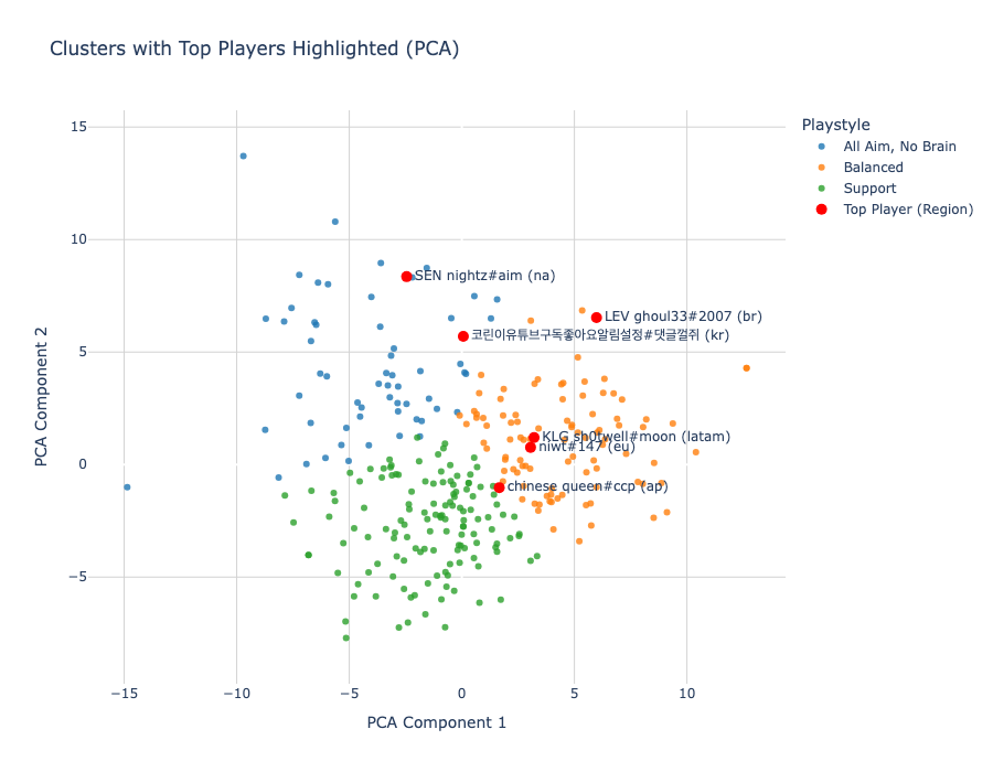
Figure 8. PCA cluster visualization
Interestingly, out of the six top players highlighted, only one fell into the Support cluster and it was the highest ranking Asia-Pacific player for this act. Similarly, there were only two AANB players, coming from North America and Korea. The rest of the highest ranking players fell under the Balanced label. Comparing mean RR values between clusters (Figure 9) shows that AANB and Balanced players find similar success in accumulating RR, whereas Support players fall behind.
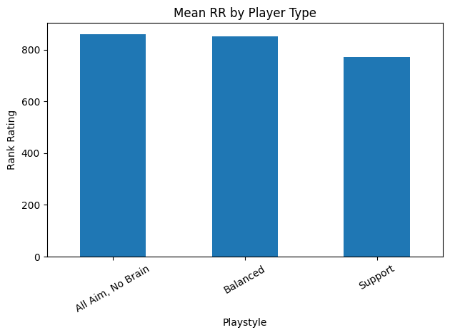
Figure 9. Mean RR by player type
In addition to visualizing the clusters on the mapped PCA space, I compared the cluster distributions within each region to understand each region’s differences in playstyles (Figure 10). The regions are sorted by % AANB in descending order, revealing that Brazil has the highest proportion of players in that cluster while Korea has the lowest by a large margin. In fact, the majority of the top 50 players in Korea fell under the Support cluster, which is known for having lower RR values than the other clusters. This explains the RR disparity found in the EDA section, which showed that the Korean region struggled to accumulate higher RR values than the rest of the world for this act.
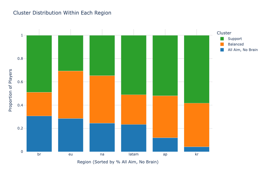
Figure 10. Cluster distribution by region
With so many Support players in the region, it’s also worthy to note that the highest ranked player from Korea fell under the AANB cluster, which suggests that AANB players can capitalize more on the abundance of support in the region. However, it is also interesting to point out that the highest rated player from Asia Pacific was a Support player, which is the complete opposite of Korea despite both of the regions sharing relatively similar cluster distributions. This implies that playstyle, while correlative, is not the primary factor for determining ranked success. To further answer that question, I moved on to predictive modeling.
8. Predictive Modeling
With the dataset cleaned and standardized, I trained a set of regression models to predict two key measures of player success: rank rating (RR) and game win percentage. The goal was twofold: (1) assess how accurately these metrics could be predicted from gameplay statistics, and (2) analyze which features contributed most strongly to the models’ predictions.
All models were trained using an 80/20 train-test split, and hyperparameters were tuned using GridSearchCV with 5-fold cross-validation. The same tuning strategy was applied to both target variables. The search grids were as follows:
- Lasso/Ridge:
- Regularization strength alpha tuned automatically via cross-validation (cv=5)
- Random Forest:
- Number of estimators chosen from 100 or 200
- Maximum depth chosen from none, 10, or 20
- Minimum samples split chosen from 2 or 5
- XGBoost:
- Number of estimators chosen from 100 or 200
- Maximum depth chosen from 3 or 6
- Learning rate chosen from 0.05 or 0.1
8.1 Predicting Rank Rating (RR)
Using RR as the target variable, the results of the four models are shown in Table 3. The linear models outperformed tree-based methods on this task, suggesting that RR may be more closely tied to linearly distributed performance metrics. Ridge performed best overall, and was used to visualize global feature importance using SHAP values.
Table 3. Evaluation of models (y = RR)
| Model Type | R² | RMSE | MAE |
|---|---|---|---|
| Lasso (L1) | 0.43 | 0.79 | 0.64 |
| Ridge (L2) | 0.47 | 0.76 | 0.63 |
| Random Forest | 0.27 | 0.90 | 0.68 |
| XGBoost | 0.31 | 0.87 | 0.68 |
To interpret the Ridge model’s predictions for rank rating (RR), I computed SHAP values across the training set and visualized them in a beeswarm plot (Figure 11) to highlight the most influential features. Surprisingly, the single most impactful variable was the number of 1v2 clutches lost, which showed a strong negative correlation with RR. This suggests that even among top-tier players, frequent failures in clutch situations are penalized more heavily than one might expect. Additional important features included thrifty rounds won, assists per round, and plants per round. Notably, while assists per round had a positive correlation with RR, total assists showed a negative one. This implies that players who contribute consistently within each round are valued more highly than those who accumulate assists across many games—reinforcing a theme seen earlier in the analysis: top-performing players tend to exhibit more impactful efficiency rather than constant support play. The negative relationship between plants per round and RR further supports this notion—suggesting that high-RR players may take on roles that prioritize fragging and round-closing impact over team objectives.
Another surprising pattern was the simultaneous positive correlation between legshots dealt and RR, and positive correlation between headshot percentage and RR—two stats that theoretically should be negatively correlated. The prominence of legshots dealt as a more important feature hints at a playstyle where damage output and pressure matter more than pristine aim statistics. This may reflect behaviors like wallbanging or suppressive utility use, especially in high-pressure situations where chip damage accumulates over time. Additionally, the model revealed a negative correlation between defensive assists per round and RR, contrasting the positive effect of assists in attacking rounds. This suggests that high RR on defense may be associated with more self-sufficient, proactive fragging, where players convert opportunities into kills rather than rely on coordinated trading. Together, these insights reveal a model of ranked success that favors decisiveness, impact per round, and opportunistic damage, rather than raw support or consistent utility contribution.
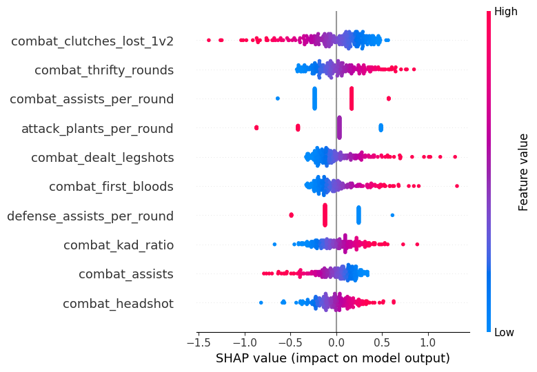
Figure 11. SHAP RR Top Features
8.2 Predicting Win Rate
While RR is the most visible measure of ranked progression, it is influenced by hidden matchmaking factors, rating adjustments, and volatility outside a player’s control that is sometimes dealt with by increasing playtime. In contrast, game win rate (WR) offers a cleaner target that directly reflects a player’s consistent ability to help their team win matches. It is less noisy, more stable over time, and arguably a more meaningful measure of player impact.
Using the same methodology, I tested four model architectures to predict win rate. The results are found in Table 4. All four models performed better with this target variable than when they were fit to predict RR (comparable due to standardization), leading to potentially more applicable insights. Among these models, XGBoost performed the best, although the results were very similar. Again, I used the best performing model to visualize feature importance using SHAP values.
Table 4. Evaluation of models (y = win rate)
| Model Type | R² | RMSE | MAE |
|---|---|---|---|
| Lasso (L1) | 0.55 | 0.61 | 0.50 |
| Ridge (L2) | 0.58 | 0.60 | 0.46 |
| Random Forest | 0.60 | 0.58 | 0.46 |
| XGBoost | 0.62 | 0.57 | 0.46 |
I visualized the feature importances in Figure 12 and found several interesting trends. Several of the top features surfaced by the XGBoost model aligned with expectations, such as KAD ratio, KAST, and deaths per match, which are all well-known indicators of consistent performance. However, a few features stood out for their more nuanced or counterintuitive contributions. For example, match duration had a strong negative correlation with win rate—suggesting that longer games tend to be less decisive or more prone to losses. This may reflect the volatility of extended matches where teams fail to close out early leads, or a higher likelihood of tilt and inconsistency over time. Interestingly, defuses also had a negative correlation with win rate. This could imply that players on frequently defusing teams may be compensating for weaker defensive positioning or trading patterns that allow plants in the first place, rather than controlling the round early.
Another intriguing observation was the rise of KAST as a top feature in the win rate model, despite it being less influential in the RR prediction task. This suggests that reliable round-to-round participation—including survival, trading, and support—is more tightly linked to team success than to individual matchmaking outcomes. Similarly, clutches (overall) showed a negative correlation with win rate, while 1v2 clutches lost also correlated negatively. This dual appearance may highlight that high clutch engagement—whether successful or not—often reflects being in disadvantageous round states to begin with, hinting at systemic team struggles. Together, these patterns underscore that winning games is not just about individual moments of impact, but about avoiding the situations where heroics are even necessary.
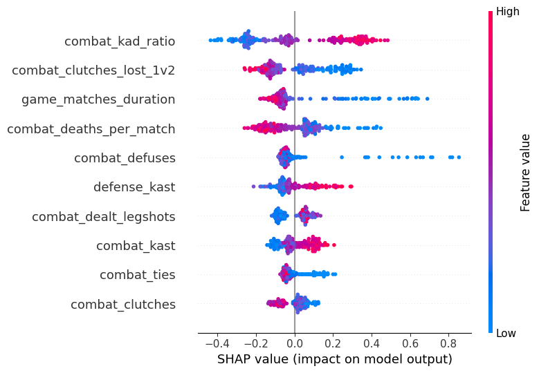
Figure 12. SHAP Win Rate Top Features
9. Personalized Evaluation
To extend the analysis beyond top-ranked leaderboard players, I applied the same PCA projection and predictive modeling techniques to evaluate myself and a group of friends using our own match data. This offered a practical lens through which to assess individual playstyles, identify statistical strengths and weaknesses, and suggest data-driven adjustments that could help improve ranked performance.
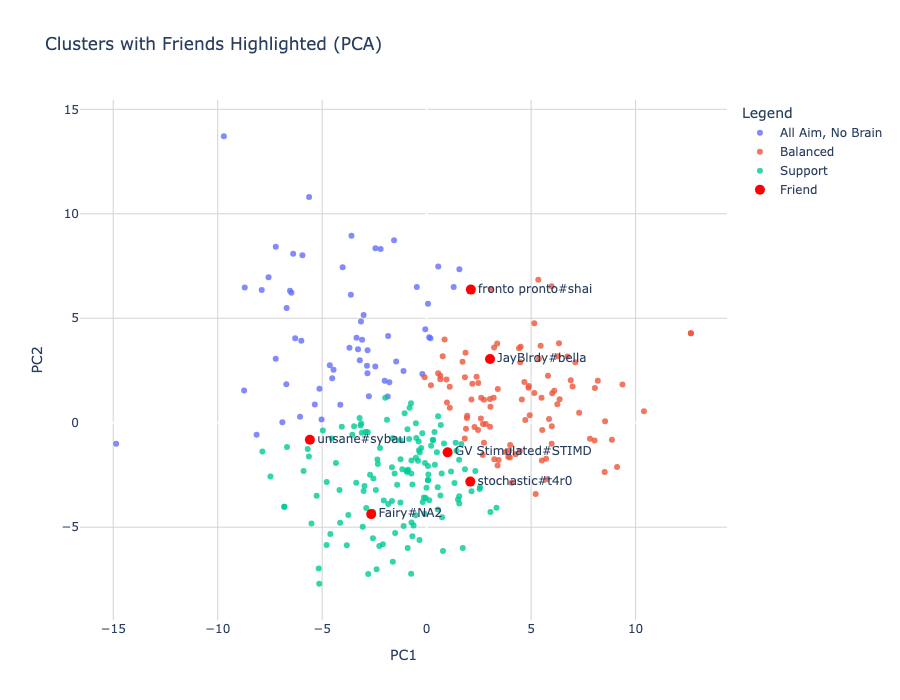
Figure 13. PCA with friends
In Figure 13, I visualized our player profiles on the same two-dimensional PCA plot used in the earlier clustering analysis. Interestingly, the majority of us fell into the Support cluster—a group characterized by stats associated with teamwork, trading, and objective play. However, two players landed within the Balanced cluster. Subjectively, these two are also the strongest players in the group, with one currently Radiant #32 in North America. This visual reinforces an earlier insight from the clustering and modeling sections: playing a highly supportive role may not be the most effective strategy for climbing in ranked, where the system tends to reward self-sufficient impact and round-defining plays more than silent consistency. For players aiming to improve their rank, this plot suggests that evolving toward a more proactive or hybrid playstyle—incorporating entry potential, clutch capability, or direct fragging power—could be a meaningful step forward.
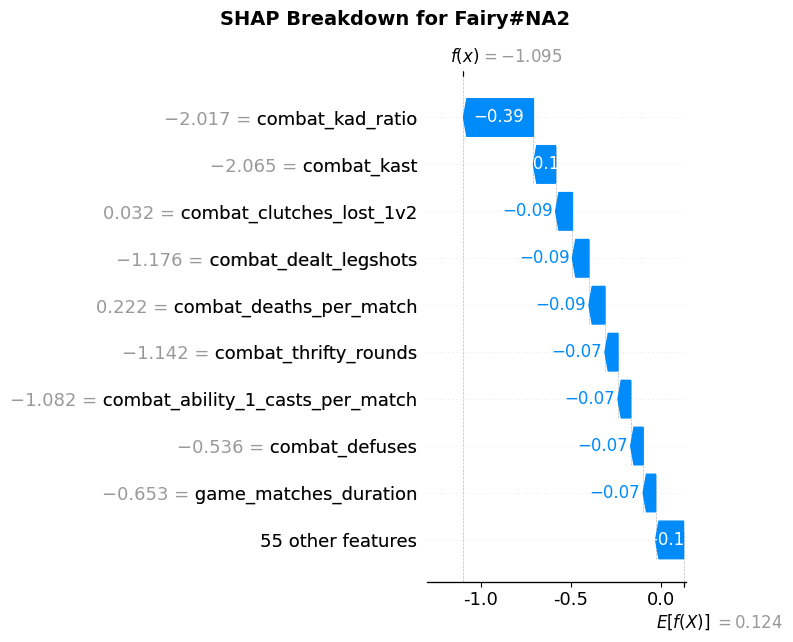
Figure 14. SHAP Breakdown for Fairy#NA2
To further personalize the evaluation, I used the XGBoost model trained on win rate to generate SHAP breakdowns for each friend. These visualizations decompose the predicted win rate for each player into individual feature contributions, highlighting which aspects of their performance helped or hurt their overall effectiveness. In the case of Fairy#NA2, Figure 14 shows that nearly all features negatively affected their predicted win rate, consistent with the fact that this player had a relatively poor act. This breakdown aligns closely with the global feature importance plot, reinforcing the model’s validity in individualized contexts. In contrast, JayBlrdy#bella also had a suboptimal predicted win rate (Figure 15), but for different reasons. His SHAP breakdown highlighted high deaths per match as a major contributor to poor performance, but also identified strengths—such as frequent first bloods and strong 1v2 clutch performance—suggesting which showcase his mechanical prowess as an entry-duelist player.
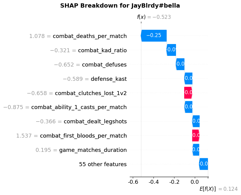
Figure 15. SHAP Breakdown for JayBlrdy#bella
Finally, fronto pronto#shai, the Radiant player in the group, showed a much stronger SHAP profile (Figure 16), with more positive than negative contributing features. His high win rate was supported by stats such as shorter match durations, strong KAD and KAST values, and a surprisingly impactful number of legshots dealt—echoing earlier findings about damage-over-precision tendencies in successful players. Altogether, this personalized SHAP approach provides not just individualized diagnostics, but also tailored, actionable insights, offering each player a clearer picture of how to evolve their playstyle in a ranked environment.
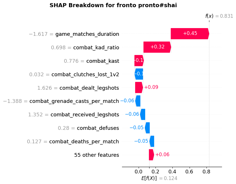
Figure 16. SHAP Breakdown for fronto pronto#shai
10. Limitations
While this analysis offers meaningful insights into the performance profiles of top-ranked VALORANT players, several limitations constrain the generalizability and scope of the results.
The most significant constraint was data access. Due to the restricted nature of Riot’s official API, I was unable to collect comprehensive match history data across the full VALORANT player population. Instead, I relied on web scraping from Tracker.gg, which itself presented challenges: CAPTCHAs, dynamic loading delays, and occasional rate-limiting errors (HTTP 429) all required careful handling. As a result, the scraping process had to be significantly slowed down, and I limited the dataset to the top 50 players from six major regions, yielding a final sample of 292 out of a possible 300 player profiles. This approach ensured consistency and quality, but significantly limited the dataset’s size and diversity.
A related issue is that the dataset focuses exclusively on the top 0.05% of players—a subset with extraordinary game sense, mechanical ability, and coordination (vstats.gg). While this made for a compelling study of elite-level play, it limits the applicability of the findings to the broader player base. Even when comparing these players to high-Immortal or Radiant players within my friend group, the performance dynamics and matchmaking environment differ enough that direct comparisons should be interpreted cautiously. Insights around optimal playstyle, feature importance, or statistical tendencies may not translate to lower or mid-tier competitive ranks, where decision-making frameworks and team dynamics vary widely.
Additionally, the use of Rank Rating (RR) as a target variable posed its own challenges. RR is a relatively noisy metric, affected not only by player performance but also by matchmaking system factors such as team composition, opponent MMR, and win/loss streak modifiers. With more data—particularly from a wider range of players and matches—some of this noise could have been mitigated through aggregation or modeling. Likewise, all data in this project comes from a single competitive act, limiting the analysis to one snapshot in time. Player performance, meta balance, and matchmaking systems evolve between acts, so longitudinal data across multiple seasons would yield more robust and generalizable insights.
Looking ahead, acquiring production access to Riot’s API or collaborating with platforms that have large-scale match data could dramatically expand the scope of this project. This would allow for population-level sampling, better representation across ranks and playstyles, and a deeper understanding of how performance traits vary not only by region and role, but also over time.
11. Conclusion
This project set out to answer a simple but important question: what distinguishes the top-ranked VALORANT players from everyone else—and how can that knowledge be applied to better understand, model, and potentially improve individual performance? By collecting and analyzing data from Tracker.gg for the top 50 players in six major regions, I explored this question from multiple angles: unsupervised clustering, supervised predictive modeling, and personalized player evaluations.
Through clustering and PCA visualization, I identified distinct playstyle archetypes among elite players—such as high-impact fraggers, well-rounded hybrids, and support-oriented teammates. Interestingly, the majority of my friends (and myself) fell into the Support cluster, which is something we’d like to work towards adjusting with data suggesting that players with more proactive or selfish statistical profiles were more successful at climbing the ranked ladder. Predictive modeling further supported these insights: while KAST and KAD ratio were among some of the top predictors of success, more niche statistics like 1v2 clutches lost, game duration, and legshots dealt seemed to hold surprisingly high importance. On the other hand, team-play metrics related to plants, defuses, and assists were negatively associated with Rank Rating (RR) and win rate—suggesting that individual impact often outweighs supportive consistency when it comes to earning RR.
Model performance was stronger when predicting win rate than RR, highlighting the noisy nature of the ranked system and the added benefit of focusing on outcome-based metrics. SHAP values offered an interpretable breakdown of feature importance at both global and individual levels, helping diagnose what players were doing well and where they could improve. Personalized SHAP analysis of my friends revealed common pitfalls (e.g., KAD ratio, 1v2 clutches lost, et cetera) and unique strengths (e.g., first bloods, clutch resilience), showing how data can power targeted, player-specific recommendations.
Despite the limitations of a small, elite-only dataset and scraping constraints, this project demonstrates the power of data science as a lens for understanding gameplay at scale. Looking forward, there are several ways to expand on this work:
- Build a web app where users can input their IGN and receive automatic performance analysis with clustering and SHAP feedback
- Add longitudinal tracking to study performance trends across multiple acts or patches
- Extend the analysis to other competitive games or compare player behavior across genres (e.g., FPS vs. MOBA)
- Apply these tools in coaching, content creation, or game balance feedback loops
Ultimately, this project blends personal passion with analytical rigor—and highlights how statistical analysis can bring clarity, direction, and even creativity to competitive gaming.
12. Sources
- Posted on:
- April 22, 2025
- Length:
- 29 minute read, 6147 words
- See Also: