Modeling Customer Behavior
s
I. Abstract
Predicting customer behavior is a crucial part of the e-commerce industry for platforms such as Fingerhut to enhance user experience and drive business. Our team leveraged the extensive dataset provided to us from Fingerhut to focus on predicting whether a customer will complete a “journey” on the company’s web page; defining a successful journey as one where the customer reaches the ‘order shipped’ event stage. After our team performed meticulous feature engineering and cleaning on the dataset, we evaluated and trained the data on several different models, such as Logistic Regression, Gradient Boosting, Neural Networks, XGBoost, and Decision Trees, finding the XGBoost model to be the most effective, achieving the highest F1 score of 73%. Although our team faced many limitations due to the extensive size of the dataset as well as our limited computing power, we believe our results to be of great value to the Fingerhut team and to have the potential to be leveraged to learn more about their customer’s behavior and evidently drive business in the coming years.
II. Introduction
In the contemporary landscape of e-commerce, Fingerhut stands out as a pioneering online retailer offering a diverse array of products ranging from electronics to housewares, apparel, and sporting goods. What distinguishes Fingerhut in the market is its unique credit model, which empowers customers, particularly those with limited or poor credit histories, to access products they might otherwise find financially challenging. Through the provision of Fingerhut credit accounts, customers can make monthly payments on purchases, thus facilitating their ability to afford desired items while simultaneously working towards rebuilding their credit profile.
For the purpose of this analysis, we have been granted access to a dataset encompassing Fingerhut’s FreshStart customer universe, i.e. customers that are allowed to make a single purchase up to their credit limit, typically ranging between $150-$200, before transitioning to a revolving line. This dataset documents key events along the customer journey, from the initial credit application to the pivotal moment of order shipment. Each customer’s trajectory is delineated by milestones, including the application for credit, the first purchase, the down payment, and the subsequent shipping of the order. Additionally, the dataset captures ancillary events such as website visits and cart additions, providing rich insights into customer behavior and engagement.
Fingerhut seeks our expertise to delve into the intricacies of customer journeys. Whether we unravel the typical trajectory a customer traverses, identify distinguishing features of a complete journey, or discern potential obstacles or deviations from the ideal path, by understanding the nuances of customer behavior, we aim to illuminate critical indicators that may signify a customer’s likelihood of a completing a successful journey.
Upon completing the data preprocessing and conducting exploratory data analysis, our team uncovered compelling insights within the data on the various event stages, timestamps, and customer journeys. Thus, we decided that pursuing a model capable of predicting whether a customer would make a purchase based on their first couple interactions on the website would both leverage the combined strengths of our team as well as provide valuable information for Fingerhut. After noting the year-over-year orders shipped decreasing in our initial data analysis, we created this model with the intention of Fingerhut leveraging it to track customer habits and utilize the insights the model provides to craft their website and user interface in a way that would guide more customers towards making a purchase and hence drive business. Our team also believes that the model could also provide Fingerhut information on why they were losing customers that were on their website, but did not make a purchase.
To do this, we must first define a successful journey as one that results in the ‘order shipped’ event, the inflection point at which a customer transitions from a closed-end, limited line to a revolving line. As many prospecting customers’ journeys end before this crucial event, analyzing when and where people lose interest can provide invaluable insights for the growth of Fingerhut’s customer base. From here, we began to perform more specific data exploration to find a model that would best work with the given data as well as how to formulate a dataset that could be fed into the model, our main goal being to provide Fingerhut with a model that could predict whether a customer would make a purchase as well as to provide insights that could combat their declining revenue year-over-year.
III. Data Preparation
The given data from Fingerhut’s team was limited, featuring a maximum of 13 unique features with some events perfectly correlating with others, such as ‘event_definition_id’ and ‘event_name’. Each row represented an individual customer event which made up a step in one of thousands of customer journeys. This dataset presented certain challenges, including duplicate rows with identical timestamps and a sequential index for journey steps that was disrupted upon removal of such duplicated rows.
To address these challenges, we undertook a series of preprocessing steps to ensure data integrity and maximize analytical potential. Firstly, we removed duplicate rows based on identical timestamps and reindexed the ‘journey_steps_until_end’ column to preserve its sequential property, ensuring consistency in journey step enumeration as shown in Figure 1.
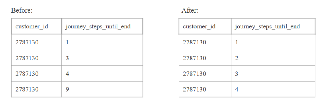
Figure 1. Transformation of the ‘journey_steps_until_end’ column
Subsequently, we transformed the data into wide format by grouping all rows by ‘customer_id’, enabling a comprehensive view of each customer’s journey across multiple dimensions. Leveraging this wide-format structure, we performed extensive feature engineering to extract insightful variables that could enable us to accurately predict customer journey success. In total, we engineered 27 novel predictors to help conduct our analysis objectives, listed and described in Appendix Table 1.
Notable features include ’num_journeys’ and ‘max_journeys’, quantifying the frequency and maximum length of customer journeys respectively. Furthermore, we delineated key milestones such as ‘first_purchase’ and ‘order_shipped’, enabling granular assessment of journey progression and success. We also leveraged temporal aspects of our data using the ‘event_timestamp’ variable, such as the creation of the ’time_in_discover’ and ’time_in_apply’ variables, shedding light on the duration spent in these specific journey stages. We explored device usage patterns through ‘initial_device’, discerning whether customers accessed Fingerhut via mobile devices or web browsers, and included lists of the beginnings of each customer’s time with Fingerhut by adding a ‘first_n_events’ column (using n=5, n=20) as well as the time delta between those events in a ‘time_since_last_event’ column. We then trained an LSTM model to generate embeddings for the ‘first_n_events’ and ‘time_since_last_event’ variables to reduce dimensionality of these variables while preserving the information within them. We hypothesized that a customer’s initial interactions with Fingerhut could drastically affect their relationship with the service, making the last two variables crucial for our analysis.
Furthermore, upon a carefully consideration while training the machine learning models, we decided to drop 8 columns from the feature engineered dataset: ‘downpayment_cleared’, ‘first_purchase’, ‘max_milestone’, ‘downpayment_received’, ‘account_activation’, and ‘customer_id’, ‘first_20_events’, and ‘time_since_last_event’. This gave us a dataset with 27 columns, in which 10 columns are embeddings resulting from ‘first_20_events’ and ‘time_since_last_event’.
Lastly, all data preparation and feature engineering procedures were replicated on both the original dataset and a 5% customer sample dataset, ensuring consistency and scalability in model training and analysis. By curating the dataset with informative features, we have laid a robust foundation for subsequent analysis and modeling.
IV. Data Exploration
There were a few things that we wanted to explore in order to learn more about our dataset. We were very interested in the proportion of customers who ultimately completed a purchase (as indicated by the ‘order shipped’ variable). We noticed that we have a very unbalanced dataset as shown in Figure 2.
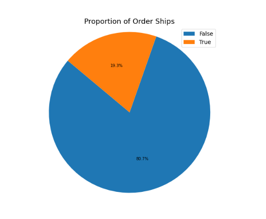
Figure 2. Proportion of customers with an Order Shipped
Taking this into consideration. This gave us an accuracy benchmark for our models of around 80%.
We also wanted to investigate the ‘discover’ variable. This variable relates to fingerhut’s advertising strategies, so we expected to see a measurable correlation in customers who interacted with fingerhut’s marketing campaigns and their likelihood to complete a purchase. We checked the proportion of customers who had and had not interacted with the ‘discover’ variable. As seen in the barplot below, we actually found no significant difference between the amount of customers who completed an order.
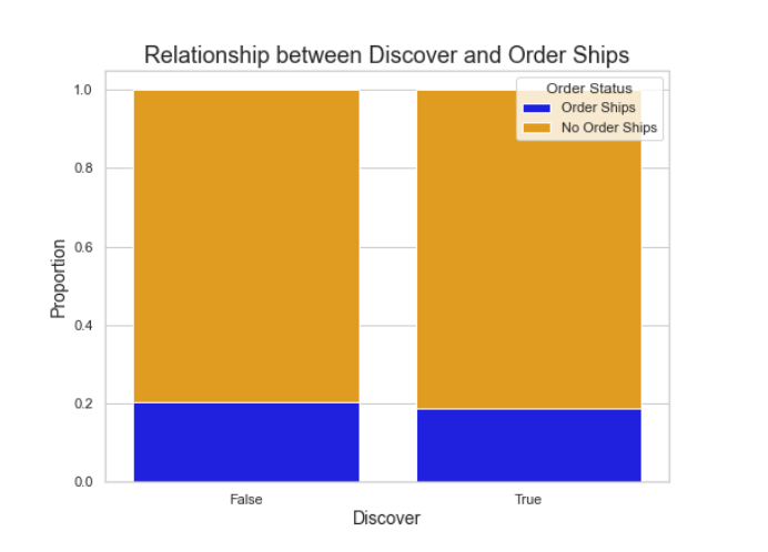
Figure 3. ‘Discover’ vs Order Shipped
Another variable we were interested in is the number of steps a customer took through their journey through the Fingerhut site. This varied dramatically for each customer. Many had only one or two steps, but there were some that had over hundreds of steps. Considering there were multiple outliers with over 1000 steps. We decided to display this distribution on a logarithmic scale. As shown in the histogram, the majority of customers had journeys that were between 10 and 100 steps.
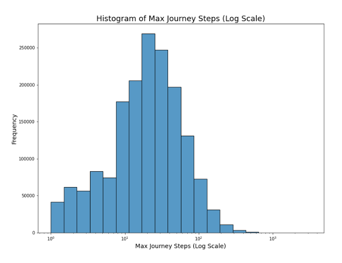
Figure 4. Max Steps per Journey (log scale)
Finally, we also noticed an interesting trend in sales. Within the year, there seems to be a large spike in sales around the end of the year in November/December. This is obviously very typical for any retailer considering the amount of shopping people do around the holidays. We also noticed a spike around March. However, the most noticeable trend that we saw was a decrease in traffic over the last 3 years.
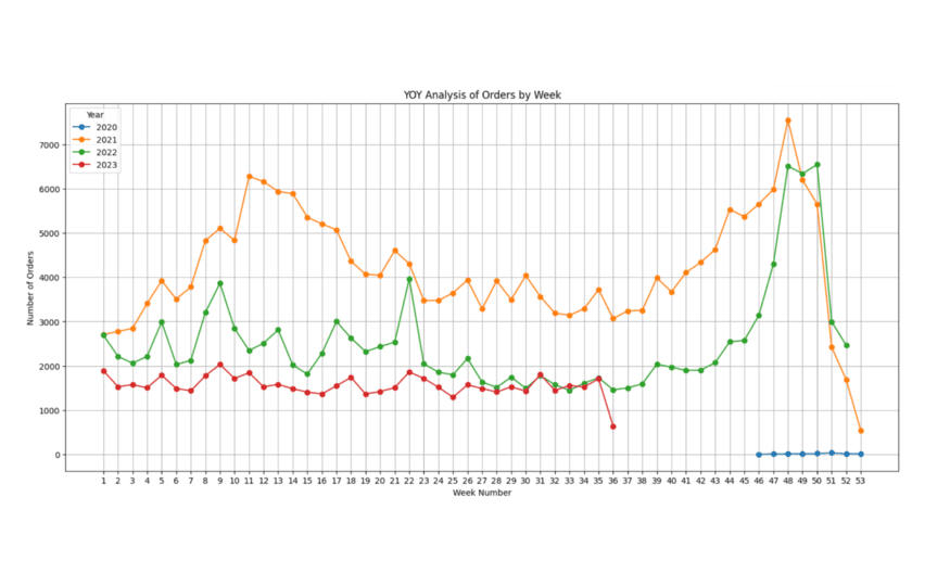
Figure 5. Weekly Order Analysis by Year
This was something that we kept in mind as we built our model, understanding that the year, as well as time-of-year, could have an impact on Fingerhut sales as well.
V. Classification Models
After delving into the wide format data set by providing a deep description of derived features, the subsequent objective was to select the model that best fitted the data and exhibited highest performance. In this section, we provide an in-depth analysis of the architectures, methodologies, and strategies adopted, which included a diverse spectrum of models ranging from statistical or boosting trees to a more abstract model such as a neural network.
An initial model testing on a proportionally preserved subset of the data revealed poor performance due to imbalanced class proportions, with 80% representing customers being unsuccessful in the ‘order_shipped’ goal and 20% those who did. To address this imbalance, two strategies, upsampling and downsampling, were employed, each with its associated risks of overfitting on the minority category or loss of valuable information. While these strategies initially improved model performance, their biases led to a decision to retain the original class proportions for realistic reporting of results.
For model training, we used the preprocessed original dataset with time embeddings, which contains 1,665,374 rows and 27 columns, of which 10 columns are the resulting embeddings from columns (‘first_20_events’ and ‘time_since_last_event’). First, we explored seven different kinds of preliminary models: Logistic Regression, Decision Tree, XGBoost, AdaBoost, Gradient Boosting, Light-GBM, and Gaussian Naive Bayes. The reason why we considered these models was because we wanted to try out different methods that use different methods for inference, for example ensemble methods and probabilistic models. Also, we used the Logistic Regression model as our benchmark. After training and testing on these seven models, we realized that out of these seven preliminary models, XGBoost had the best performance (with LGBM being the second), while the other six preliminary models suffered from their low F1 scores. Thus, we decided to move on to both tuning the hyperparameters for the XGBoost model as well as designing new complex models for downstream classification tasks. For tuning, we utilized the Optuna library to tune the specific hyperparameters: ‘n_estimators’, ‘max_depth’, ‘learning_rate’, ‘subsample’, ‘gamma’, ‘scale_pos_weight’, ‘reg_alpha’, and ‘reg_lambda’. This library utilizes a Bayesian Optimization approach to find the best and optimal hyperparameters for our models, allowing us to decrease the number of training iterations.
On the other hand, in an attempt to increase the metrics that previous models were showing up, we designed a Neural Network in order to see if this kind of algorithm could extract uncovered patterns in the data and leverage them in order to get a higher accuracy and f1 score. This Neural Network was designed with the following architecture: five fully connected layers with ReLU activations and Dropouts in between, L2 regularization, and finally activated by a Sigmoid function. Before feeding the training data into the Neural Network, we also calculated the corresponding weights for each label.
Lastly, we designed a framework that first clusters the data points into one of the two clusters, then trained and tested separate XGBoost models. However, due to its worse performance, we have decided to omit this design.
VI. Results
It is worth mentioning that the way we assess our models is really important while choosing the best model, in this regard we can see that metrics play a crucial role in the measure of performance. Therefore, after training our preliminary models we calculated initially the accuracy metric which is the standard measure for model performance assessment. The results can be seen in the following plot:
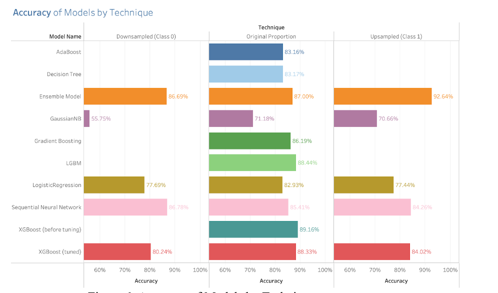
Figure 6. Accuracy of Models by Technique
The accuracy scores are divided into three different categories: the scores for the models trained with the downsampled data, the scores with the models trained with upsampled data, and the scores for the models trained with the original proportion of data. But the analysis over the scores are not going to be performed over these results and this is due to the fact that certain metrics can lead to misleading results due to the nature of the data. In this regard, the accuracy metric is not always a reliable metric for evaluating the model performance and particularly in a high unbalanced data set which is our case. Instead, the F1 score stands out as a robust measure. The F1 score is calculated using the harmonic mean of precision and recall where its formula is
F1 = 2 * (precision * recall) / (precision + recall)
In this sense, the model evaluation was entirely focused on improving the F1 score metric, which was the one that trustworthy demonstrated the real performance of the models. The following is the plot that contains the F1 scores of the models:
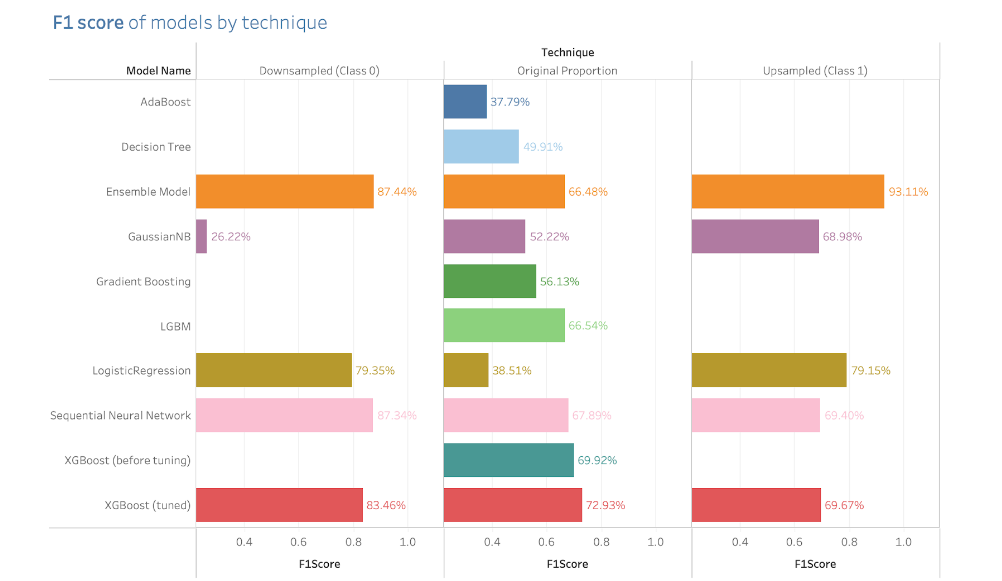
Figure 7. F1 Scores by Technique
For the downsampling scores, it is notable that there were models with an outstanding performance such as the Voting Ensemble Model or the Neural Network or even more noticeable, the Voting Ensemble Model while working with the upsampling technique. Despite that all these performances were all good, the results don’t represent a very good representation in a real scenario, but we think it is worthwhile including them in order to contrast the performances if the data were all balanced.
From the plot above, focusing on the scores for the original proportion, the 4 models with best F1 scores were the XGBoost (tuned), Neural Network, Light-GBM, and Voting Ensemble model. The naive XGBoost (before tuning) achieved an accuracy of 89.163% and a F1 score of 69.916%, and the naive LGBM achieved an accuracy of 88.438%, and a F1 score of 66.539%. These two models performed reasonably well, but as mentioned in the previous part, we believed that the XGBoost can be further improved in terms of its F1 score, especially its ability to correctly identify label 1. In addition, the accuracies and f1 score of each model is listed in Figure 8 below.
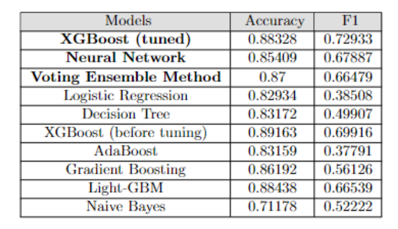
Figure 8. Accuracy and F1 Score of Models
For the tuning of the XGBoost model, we aimed to increase the F1 score instead of the accuracy, as we believed that the model’s ability to correctly identify label 1 is more important than its whole accuracy. The resulting score for the fine tuned XGBoost model is: 88.328% in accuracy and 72.933% in F1 score. Even though the accuracy of XGBoost is lower than the original by around 0.8%, we believe that this is a good tradeoff for the F1 score, which is almost 3% higher than the original one. We also plotted out the feature importance of the fine tuned XGBoost Model. From the graph, we can see that the top 5 most important features are ‘initial_decive’, ‘event_embedding_3’, ‘most_repeated_event’, ‘has_prospecting’, and ‘event_embedding_4’.
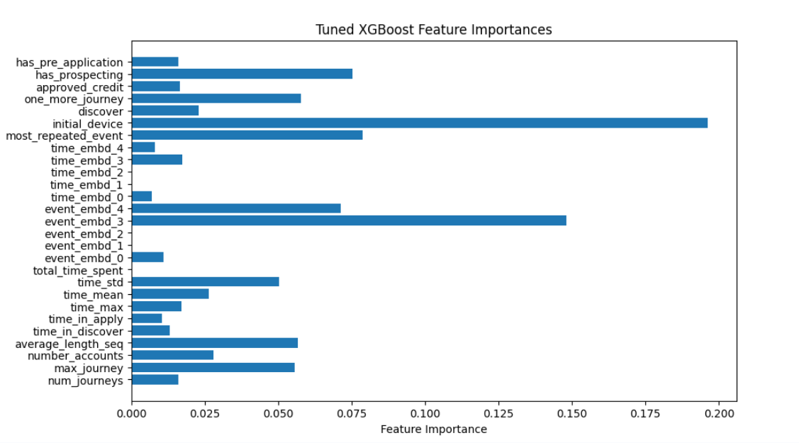
Figure 9. Feature Importances - XGBoost
For our Neural Network we had to take into consideration the proportion of classes in our data, and so we used while fitting the model the following class weights : {0 : 0.62, 1 : 2.60}. Consequently the model was trained over 5 epochs, utilizing the Adam optimizer algorithm and the binary cross-entropy as our objective function to optimize, as the accuracy is the metric of evaluation by default, we had to work with it.
In addition, we plotted out the confusion matrices for XGBoost (before tuning), XGBoost (after tuning), and Neural Network. The plots are displayed below. From the confusion matrices, we can see that both the fine-tuned XGBoost model and the Neural Network outperformed the original XGBoost in their performance of the identifying customers who will have their orders shipped (label 1 customers). Specifically, the XGBoost before tuning correctly identified 65.394% of label 1 customers, while the tuned XGBoost correctly identified 81.665% , and the Neural Network correctly identified 94.129% (both XGBoost and Neural Network have less type II errors). Note that this comes with a price: both the fine tuned XGBoost and the Neural Network performed worse in identifying label 0 customers by mistakenly identifying them as label 1. However, we believe that this is a good tradeoff since the losses of providing advertisements / incentives to customers who are predicted to finish the whole journey would likely be way less than the losses of losing real customers who are going to finish the journey.
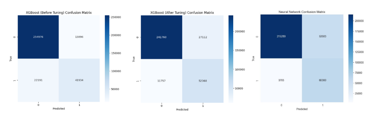
Figure 10. Confusion Matrices
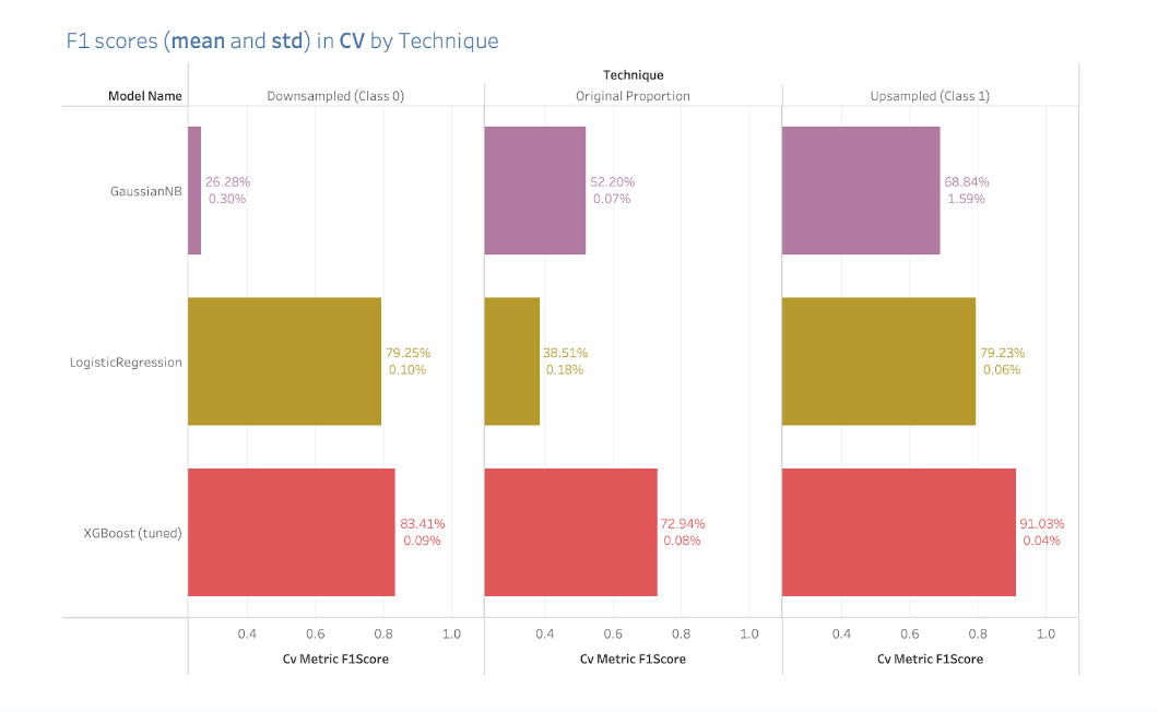
Figure 11. F1 Scores via Cross-Validation
Finally this last plot shows us the results using the Cross Validation technique for these three different models along the three different techniques used in the project. We are focusing on the original proportion and as we can observe there is a huge difference between the results that XGBoost obtained compared to the GaussianNB and the Logistic Regression. This is a very reliable technique that allows us to verify that indeed the metrics obtained in just one simple train test split were actual metrics. Moreover, the percentage below represents the standard deviation of the means in the f1 scores and in this case is very small which tells us that all these training realizations of the XGBoost model across the 5 splits used in the CV technique had very similar results.
VII. Conclusion
The results of our modeling and analysis reveal that we are able to create a model that can predict whether a customer will purchase an item through the website based on the first 20 events on the website with an F1 score of 72.93%. This achievement marks a significant step towards understanding the customer behavior and, we hope, paves the way for Fingerhut to derive further insights and analyses to help the company grow in the future.
However, although the 72.93% accuracy is promising, our team acknowledges different constraints and limitations that we faced as well as areas for improvement in the data and modeling that could potentially allow us to yield even better results. A major limitation that our team faced stemmed from the immense volume of the original dataset matched with our limited computing power. The original dataset contained 64,911,906 rows of data. Processing the entire dataset for cleaning alone required upwards of three hours. Thus, any iterative adjustments or tests we wanted to perform would cause a similarly extensive duration, making the process of modeling, analyzing, cleaning, and training extremely time consuming. Although there was a smaller sample dataset available, which was 5% the size of the original dataset, this smaller dataset introduces many significant risks, such as loss of granularity, overfitting of the model, and omission of outliers and critical events. Our solution to this limitation involved utilizing the smaller dataset for initial training, cleaning, and analysis, followed by running our end product on the entire dataset. Although we yielded promising results, our team believes that access to stronger computing power or a more manageable dataset would allow us to enhance the predictive accuracy of our model even further and make further analysis regarding customer behavior.
Our team also identified future steps that could be taken to potentially improve the accuracy and fully explore the potential of the data. Due to clustering models’ ability to group the data in an unsupervised manner, we believe that this could help yield more accurate results by allowing for customer segmentation through identifying distinct groups of customers based on their behavior and interactions with the web page. Additionally, the grouping aspect could be utilized to help feature engineering and potentially help improve the accuracy of the models by providing more data on customer behavior patterns. The models we utilized in our project are more aimed towards predicting outcomes based on input data. However, clustering could help in discovering new structures and similarities in the data that our models were unable to detect, hence increasing the accuracy and revealing more about Fingerhut customer trends.
Overall, our research provides Fingerhut with a model that is designed to predict whether a customer will purchase an item, which can be leveraged to learn more about their customers as well as their website to find ways to increase orders and evidently drive business. By analyzing patterns and trends within the first interactions of customers on the website, our model opens the door for Fingerhut to not only identify critical parts of the website that can influence purchasing decisions, but also increase the ordering rates.
VIII. Reference
Harrison, M. (March 21, 2023). Effective XGBoost: Optimizing, Tuning, Understanding, and Deploying Classification Models (Treading on Python). MetaSnake.
IX. Appendix
Appendix Table 1: Engineered Variables
| Variable | Description |
|---|---|
| num_journeys | Number of journeys per customer |
| max_journeys | Max steps in a customer’s journey |
| discover | Customer interacted with ‘discover’ |
| number_accounts | Number of account IDs per customer |
| more_one_journey | Whether customer had multiple journeys |
| repeated_event | Most repeated event |
| avg_length_seq | Average journey length |
| has_prospecting | Experienced ‘prospecting’ event |
| has_pre_application | Experienced ‘pre application’ event |
| approved_credit | Achieved ‘approved_credit’ milestone |
| first_purchase | Achieved ‘first_purchase’ milestone |
| account_activation | Achieved ‘account_activation’ milestone |
| downpayment_received | Achieved ‘downpayment_received’ milestone |
| downpayment_cleared | Achieved ‘downpayment_cleared’ milestone |
| order_ships | Achieved ‘order_ships’ milestone |
| max_milestone | Highest milestone reached |
| initial_device | First device used |
| time_in_discover | Time spent in ‘discover’ |
| time_in_apply | Time spent in ‘apply’ |
| first_n_events | List of first n events (n=5, 20) |
| time_since_last_event | Time delta between n events |
| total_time_spent | Time from 1st to nth event |
| time_mean | Mean time between events |
| time_std | Std dev of time between events |
| time_max | Max time between two events |
- Posted on:
- March 18, 2024
- Length:
- 18 minute read, 3731 words